Covariance Estimations
Overview
With every odometry message, we estimate the current standard deviation (covariances) so that users can assess the reliability of the provided position data. The estimates are updated continuously using all available sensor inputs. This allows for the quality and availability of measurements to be directly reflected in the covariance.
The following messages contain covariance estimates:
Format
The covariance values contained in the FP_A-ODOM* messages can be formatted as covariance matrices. One matrix includes the covariances for the position and heading while another matrix displays the deviation estimate of the velocity.
The matrices always have the following attributes:
The matrices are symmetrical, such that, for example,
is the same as
A covariance matrix is always a positive-semidefinite matrix and therefore the main diagonal is nonnegative
The units of the covariances are as follows:
Position covariance:
Orientation covariance:
Velocity covariance:
The shape of the position and orientation covariance matrix has the following shape:
where
The covariance matrix for position and orientation is a block matrix in which the upper right and lower left blocks are zero.
The shape of the velocity’s covariance matrix has the following shape:
Expected Behavior:
Expected Behavior:
The covariance is influenced by measurements from all available data sources, including GNSS, IMU, visual features, wheel speed, and any other measurement input. The impact of each data source on the covariance depends on several factors, such as the resolution of the data, the quality of the measurements, sensor calibration, biases, and the temporal correlation between measurements.
Example
Consider the following scenarios to illustrate this:
A car is driving in open-sky conditions. Both GNSS sensors have an RTK fix, so the system receives high-accuracy (i.e., low variance) position measurements. These measurements dominate the covariance estimator, resulting in a low output covariance.
The car now enters a tunnel and GNSS reception is lost, noisy IMU measurements are integrated, causing the covariance to increase gradually. The fusion system tracks visual features, which helps slow the rate of increase, but the high vehicle velocity and low feature environment limits the tracking length of these features. Additionally, the wheel speed sensor provides reliable longitudinal velocity data, helping to constrain the position covariance in the longitudinal direction.
The car exits the tunnel but the road is lined with trees, so GNSS availability is limited. The sensor receives positioning data, but of low accuracy (i.e., high variance). The GNSS variance is larger than the current longitudinal position variance but smaller than the current lateral position variance. As a result, the lateral component of the estimated covariance will decrease significantly, whereas the longitudinal component only reduces slightly.
The car enters an open-sky area. The output covariance is again dominated by the GNSS variance and is reduced immediately.
Note that in this example, GNSS is the only absolute measurement, therefore, as soon as there is no GNSS, the uncertainty in the estimate will grow continuously (i.e., it is unbounded).
Common Questions
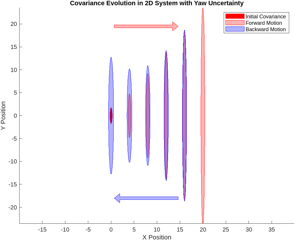
If there is some yaw uncertainty when entering an outage, then moving inside the outage will increase the position covariance in the directions orthogonal to the motion (i.e., integrating motion with heading uncertainty will result in lateral position uncertainty). If we move closer to where we entered the outage, we can “recover” some of the position accuracy we lost due to uncertainty in orientation.
See the results of passing a simple 2D system passing through a Kalman filter with no measurements in the diagram below. The system starts off facing in the positive x direction and moves forward. The covariance increases laterally, both due to process noise and due to initial yaw uncertainty. As it moves backward, some of the position accuracy lost due to yaw uncertainty can be recovered.
Covariance Evolution in 2D System with Yaw Uncertainty