GNSS statistics (gnss_stats)

Objectives

Evaluate the overall performance of the GNSS receivers.
Provide an overview of the RTK fix quality achieved by the GNSS receivers and the information they used to achieve it (e.g., satellites and signals seen or tracked).
Evaluate the quality of the baseline estimate between the two GNSS antennas and observe if the estimation passed the baseline check to initialize or re-fix the Vision-RTK 2’s position.
Analyze the reported position variance of the GNSS receivers to identify issues in the position estimate.
Ensure the GNSS receivers have an average CN0 above 42 dBHz across all signals.
Determine if the GNSS antennas have a proper view of the sky or if an object obstructs the GNSS signals.

Explanation

The GNSS statistics file allows the user to evaluate the performance of the GNSS receivers, including GNSS fix quality, estimated baseline between the GNSS antennas, average signal-to-noise ratio (CN0), position variance, number of signals and satellites, lock time for each satellite, and elevation angle analysis.

The first plot of the GNSS file presents the GNSS fix quality. For the Fusion engine to initialize, the sensor must achieve an RTK-fixed state on both GNSS receivers. The available GNSS fix types are:

Value	Fix type	Description
0	Unknown	The receiver has no satellite signals.
1	No fix	The receiver does not have enough satellite signals.
2	Dead reckoning	No satellite signals are available, but dead reckoning is enabled.
3	Time	The receiver has received time information only.
4	Single 2D	Autonomous GNSS fix with very few available satellite signals.
5	Single 3D	Autonomous GNSS fix, typically in situations with no correction data or in outages.
6	Single 3D - DR	Autonomous GNSS fix with dead reckoning.
7	RTK float	RTK with ambiguities not fully solved.
8	RTK fixed	RTK with ambiguities fully solved.
9	RTK float - DR	RTK with ambiguities not fully solved and dead reckoning.
10	RTK fixed - DR	RTK with ambiguities fully solved and dead reckoning.

The second plot presents the estimated baseline between the two GNSS antennas. In other words, it shows the distance calculated between the estimated positions of both GNSS receivers. The dotted line presents the user's baseline input, estimated from the GNSS extrinsics. The input baseline must be accurate to the millimeter level, as it serves as a reference for the Fusion engine to determine when the reported position of the GNSS receivers is drifting, or the quality of the RTK fixed measurement is low.

The third plot presents the baseline check value for each GNSS epoch and the average moving window value for the baseline check. The baseline check must pass for at least 3 seconds for the sensor to initialize.

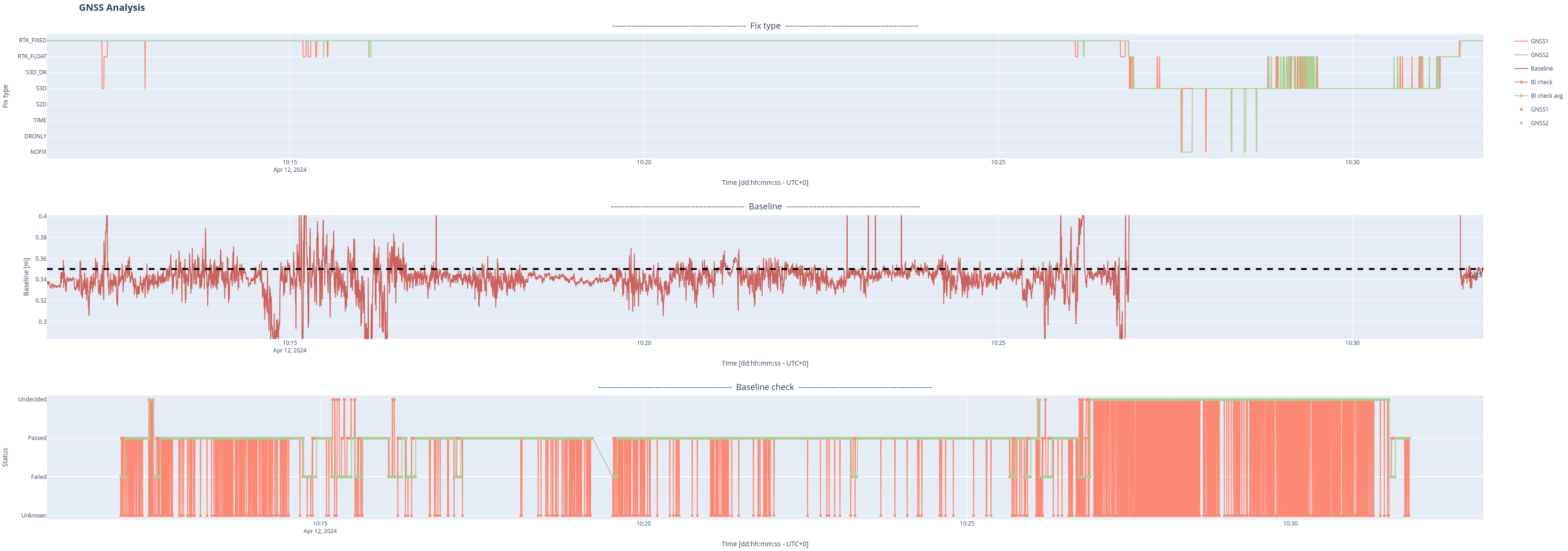
**Fig. 1:** GNSS fix type, estimated baseline, and baseline check plots.

The fourth plot presents the reported position variance of the GNSS receivers. Although less accurate than the reported covariance of the Fusion engine, it serves as a metric to evaluate when the Fusion engine should not trust the GNSS measurements. This plot is one of multiple tools that helps the user assess whether severe multi-pathing impacted the position estimate of the GNSS receivers and the Fusion engine.

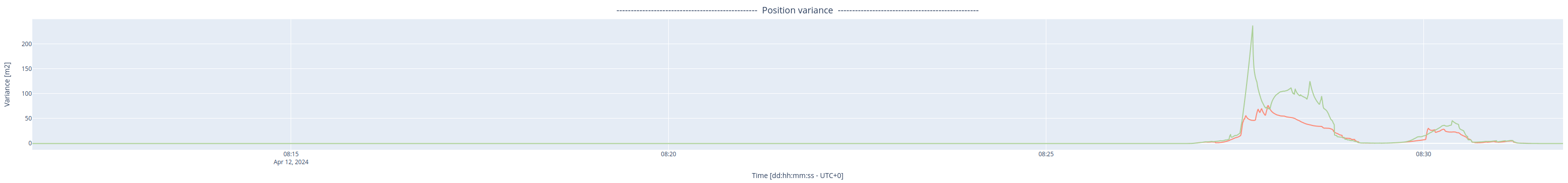
**Fig. 2:** Reported position variance of the GNSS receivers.

The fifth plot presents the average CN0 histogram throughout the recording, as shown in Fig. 3. This plot gives an overall view of the cumulative signal-to-noise ratio of all GNSS signals. Note that if most of the recording was performed inside GNSS outages, then the histogram will be shifted to the left, as the available signals will be significantly weaker throughout the recording.

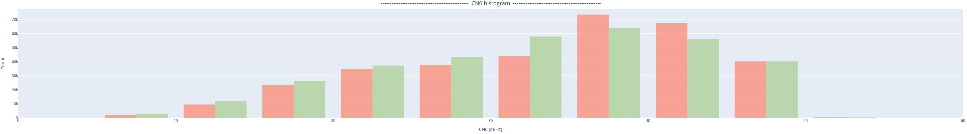
**Fig. 3:** Average CN0 histogram throughout the recording.

The sixth plot presents a time series of the average CN0 of all available signals in each GNSS epoch, as shown in Fig. 4. Small fluctuations in the average CN0 value are expected due to shadowing and multi-pathing effects. However, the user should not observe significant drops in this plot.

The seventh plot presents a similar time series with a threshold to only average signals above 40 dBHz. This plot allows for analyzing the performance of the GNSS signals with the best signal-to-noise ratio, discarding the effects of weaker GNSS signals.

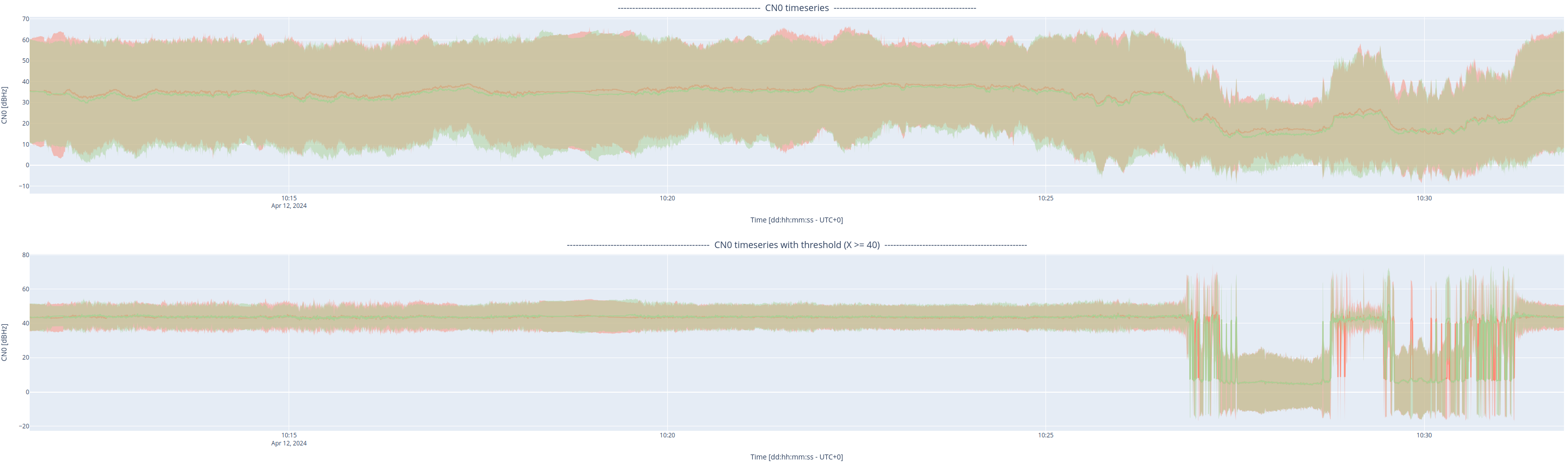
**Fig. 4:** Time series of the average CN0 of all available signals (with and without a threshold).

The following three plots allow the user to analyze the information received by the GNSS receivers and determine if the sensor has good observability of the GNSS satellites and their signals throughout the recording. They are also a tool to assess whether the location of the GNSS antennas is adequate (e.g., no objects obstruct their view) and whether any electromagnetic interference or multi-pathing effects affect the GNSS signals. In summary, these plots present the following information:

The eighth plot shows a time series with the number of GNSS signals each receiver tracks.
The ninth plot shows a time series with the number of GNSS satellites each receiver sees.
The tenth plot shows a time series with the number of used GNSS satellites for each GNSS receiver.

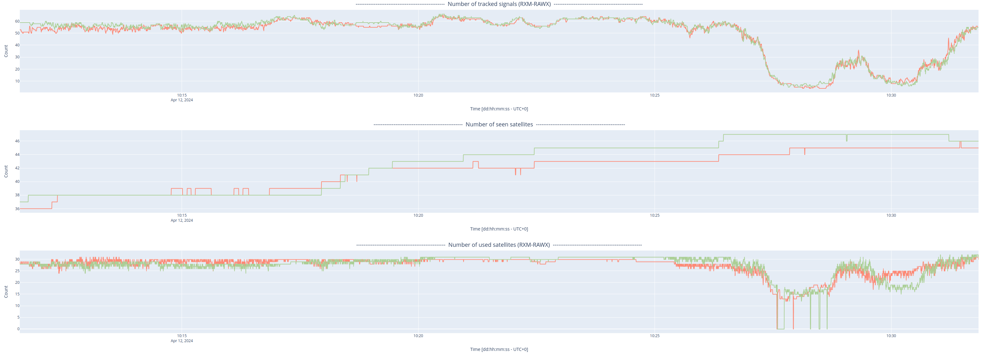
**Fig. 5:** Number of tracked GNSS signals and seen/used satellites.

The eleventh plot showcases some statistics (i.e., mean and standard distribution) about the lock time of the GNSS receivers for all tracked signals. The lock time signifies how long the GNSS receiver has been tracking the corresponding signal.

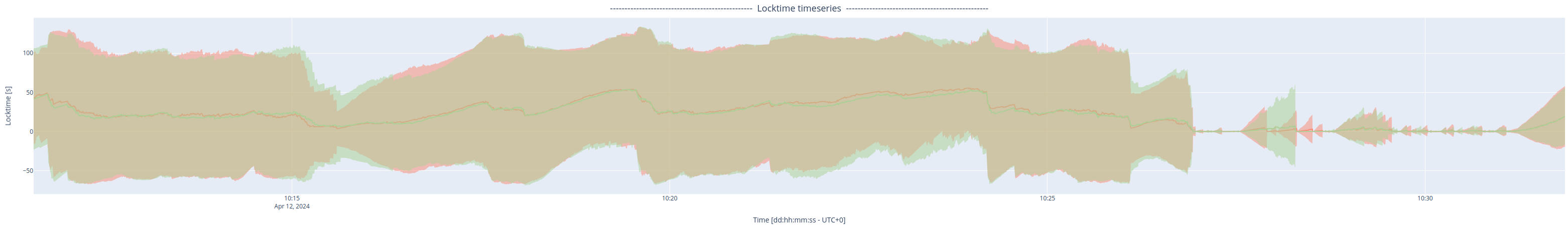
**Fig. 6:** Average lock time for each GNSS receiver.

The twelfth and thirteenth plots present a boxplot of the signal-to-noise ratio of the GNSS receivers (i.e., C/N0) vs. the elevation angle of the antennas for each L-band. The L1 band operates at a frequency of 1575.42 MHz, whereas L2 operates at 1227.60 MHz. This plot helps detect possible obstructions to the GNSS antennas and evaluate their sky visibility.

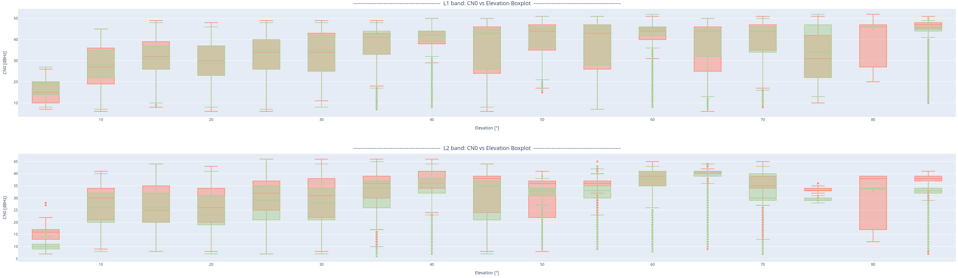
**Fig. 7:** CN0 vs. elevation boxplot per L-band for each GNSS receiver.

Example HTML:

gnss_stats.html

Expected results

Ideally, the estimated baseline should be accurate when both receivers are under RTK fixed conditions. However, it is known that the GNSS receivers can sometimes experience a 'false RTK fixed'. Thus, the user cannot entirely rely on the GNSS fix quality to assess performance. For the user to evaluate the sensor's performance, it is crucial to correlate the GNSS fix quality with the baseline check and the reported covariances.
When operating under RTK fixed conditions, the baseline check should always pass. Ensuring the input GNSS extrinsics are accurate is crucial, as any discrepancy can lead to a failed baseline check. In addition, ensure the GNSS antennas are not obstructed by obstacles or affected by electromagnetic noise and that the selected basestation is nearby (less than 25 km away).
If the baseline check fails, the Vision-RTK 2's position output will not experience a jump.
Under good GNSS conditions, the reported position variance of the GNSS receivers is expected to be under 0.001 m².
Under good GNSS conditions, the CN0 of most signals is expected to be above 42 dBHz. This value is necessary for the best positioning performance. Thus, for a recording where most of the operation was under good GNSS conditions, the histogram should show that most signals were above 42 dBHz.
The average CN0 should only drop below 42 dBHz when entering a GNSS outage. To recognize a GNSS outage, the user can correlate the information reported in the time series with the fix quality plot.
Under good GNSS conditions, the user should expect the GNSS receivers to track an average of above 50 signals. The user can notice that the number of tracked signals drops significantly after entering a GNSS outage, and it takes a couple of seconds for the GNSS receiver to start tracking them again in open-sky scenarios as it needs to regain complete visibility of them.
Under good GNSS conditions, the user should expect the GNSS receiver to observe an average of more than 30 satellites at all times. Unless the sensor enters a complete GNSS outage, the number of seen satellites is expected to drop very slowly.
Under good GNSS conditions, the receiver should use data from more than 25 satellites. Even though more satellites can be observed at a given time, unless the quality of their signals is sufficient, these satellites will not be employed by the GNSS receivers or the Fusion engine. For this same reason, the number of used satellites is almost always expected to be lower than that of seen satellites.
Under good GNSS conditions, the average lock time should always be above 20 seconds. Under RTK float conditions, the lock time should exceed 10 seconds unless the platform just left a GNSS outage.
The median CN0 for most elevations on both L-bands should be above 25 degrees. A lower value at any point could indicate an obstacle blocking the reception of GNSS signals at that elevation.

Examples

In GNSS-degraded scenarios, the reported baseline might be wrong by several meters, which can affect the scale of the plot, as shown in Fig. 6. You can always zoom in on the Y-axis only to aid in visualizing the performance of the baseline estimate when the sensor is under RTK fixed conditions.

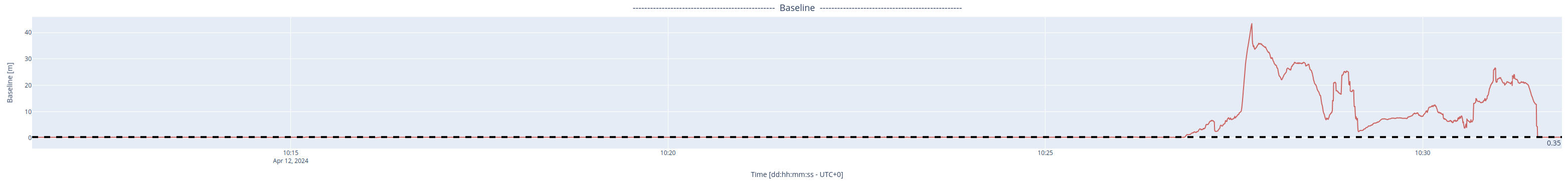
**Fig. 8:** Estimated baseline plot without zooming in on the Y-axis.

Similarly, the position variance may increase significantly in GNSS outages. The user can employ the same tool to zoom in and visualize the position variance under good RTK conditions, as shown in Fig. 7.

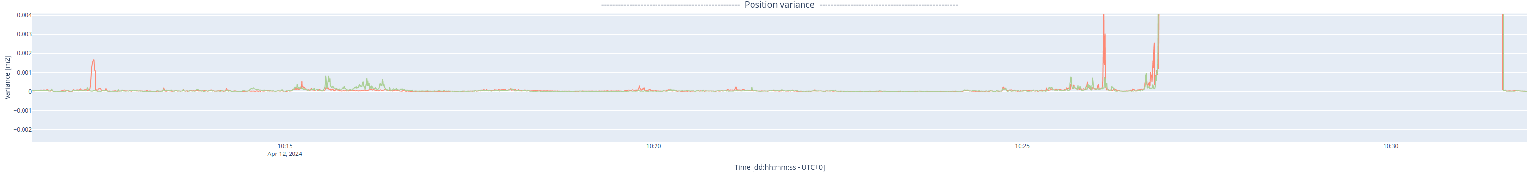
**Fig. 9:** Position variance plot zooming in on the Y-axis.

Under ideal GNSS conditions, the user should see a clear trend on the average CN0 histogram, where most of the GNSS signals are clearly situated above 40 dBHz, as shown in Fig. 10.

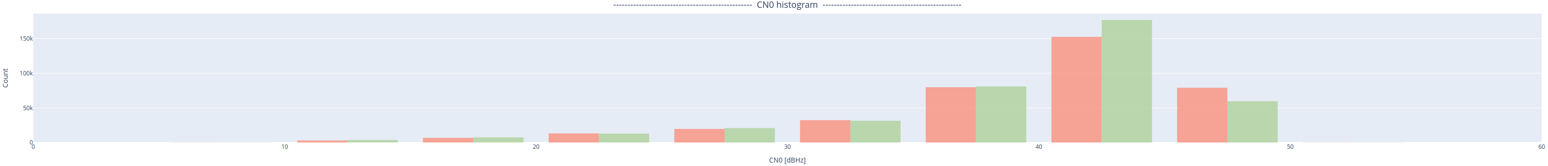
**Fig. 10:** Average CN0 histogram for a car operating on the highway.

In addition, the reported position variance of both GNSS receivers should be at all times lower than 0.001m², as shown in Fig. 11.

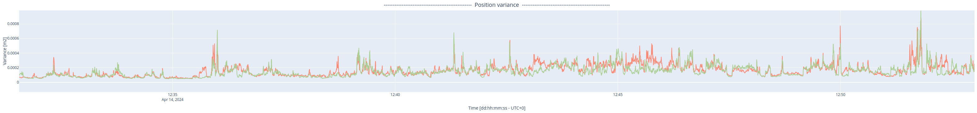
**Fig. 11:** Reported position variance of the GNSS receivers for a car operating on the highway.

When entering a GNSS outage, the estimated baseline might present a "spike", where the baseline is hundreds of meters, as shown in Fig. 12. This is the expected behavior of the GNSS receivers.

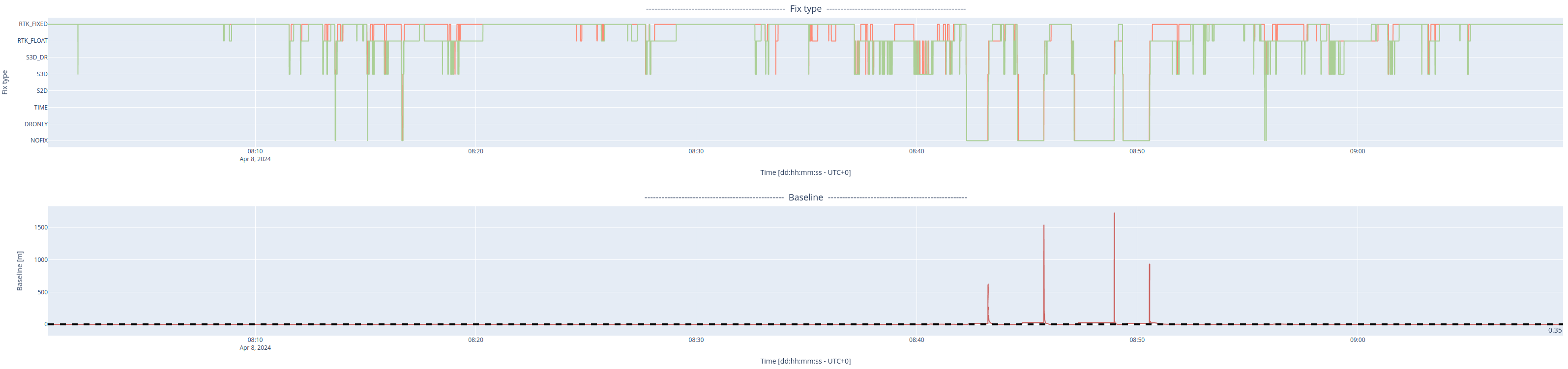
**Fig. 12:** Spikes in the estimated baseline of the GNSS receivers when entering a GNSS outage.

Similarly, during GNSS outages, the user may observe that the number of tracked GNSS signals and the number of used GNSS satellites drops significantly. However, the number of seen GNSS satellites remains mostly the same unless a very long GNSS outage is observed. Even though more satellites can be observed at a given time, because they are of low quality, these satellites will not be employed by the GNSS receivers, as shown in Fig. 13.

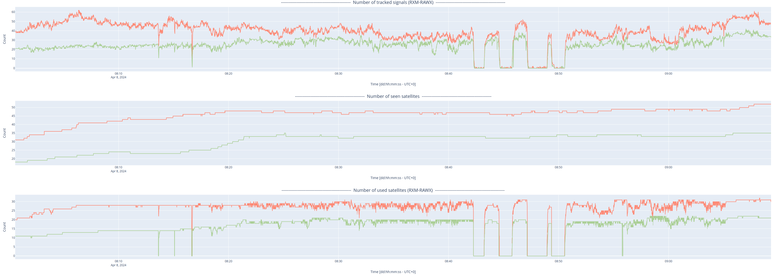
**Fig. 13:** Number of tracked GNSS signals and seen/used satellites during a GNSS outage.

Moreover, because most of this recording is under degraded GNSS conditions, the user can observe that the average CN0 histogram presents most signals with the signal-to-noise ratio skewed to the left of the plot, as their cumulative power has been significantly reduced.

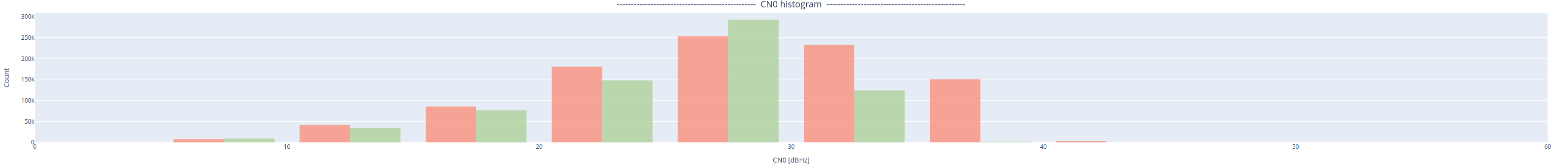
**Fig. 14:** Average CN0 histogram when the receivers are under degraded GNSS conditions.

Further analysis

If the GNSS receivers experience issues obtaining an RTK fixed status or the estimated baseline is wrong under RTK fixed conditions, verify that the selected basestation is less than 15 km from the rover. The sensor might experience degraded performance if the selected RTK basestation is slightly far away (> 15 km). The sensor will experience degraded performance and difficulties computing an RTK-fixed solution if the basestation is excessively far away (> 25 km). In this case, please choose a different NTRIP mountpoint or re-connect to the VRS service.
If the signal-to-noise ratio is low throughout the recording (i.e., CN0 under 42 dBHz), check the integrity of the GNSS cables and the power supply to the GNSS antennas, and ensure no objects are obstructing the GNSS antennas' view or any electromagnetic interference is affecting them.
If the CN0 vs. elevation boxplot presents a low signal-to-noise ratio at any angle, it is worth analyzing if any objects or structural pieces are blocking the visibility of the GNSS signals at that angle.
If the GNSS receivers' reported position variance is high at all times, even under RTK fixed conditions, then the receivers might be experiencing severe multi-pathing.