GNSS EMI analysis (gnss_emi)
Objectives
Evaluate the overall performance of the GNSS receivers.
Evaluate the quality of the baseline estimate between the two GNSS antennas and observe if the estimation passed the baseline check to initialize or re-fix the Vision-RTK 2’s position.
Determine if there is a source of electromagnetic interference (EMI) affecting the GNSS antennas, which would impact the reception of the L-bands in the GNSS receivers.
Explanation
The GNSS EMI analysis file allows the user to evaluate the performance of the GNSS receivers, including GNSS fix quality and estimated baseline between the GNSS antennas. The user can also visualize the spectrum graph for each L-band of the GNSS receiver to detect possible sources of electromagnetic interference and determine their impact on the raw GNSS signals.
The first plot of the GNSS file presents the GNSS fix quality. For the Fusion engine to initialize, the sensor must achieve an RTK-fixed state on both GNSS receivers. The available GNSS fix types are:
Value | Fix type | Description |
|---|---|---|
0 | Unknown | The receiver has no satellite signals. |
1 | No fix | The receiver does not have enough satellite signals. |
2 | Dead reckoning | No satellite signals are available, but dead reckoning is enabled. |
3 | Time | The receiver has received time information only. |
4 | Single 2D | Autonomous GNSS fix with very few available satellite signals. |
5 | Single 3D | Autonomous GNSS fix, typically in situations with no correction data or in outages. |
6 | Single 3D - DR | Autonomous GNSS fix with dead reckoning. |
7 | RTK float | RTK with ambiguities not fully solved. |
8 | RTK fixed | RTK with ambiguities fully solved. |
9 | RTK float - DR | RTK with ambiguities not fully solved and dead reckoning. |
10 | RTK fixed - DR | RTK with ambiguities fully solved and dead reckoning. |
The second plot presents the estimated baseline between the two GNSS antennas. In other words, it shows the distance calculated between the estimated positions of both GNSS receivers. The dotted line presents the user's baseline input, estimated from the GNSS extrinsics. The input baseline must be accurate to the millimeter level, as it serves as a reference for the Fusion engine to determine when the reported position of the GNSS receivers is drifting, or the quality of the RTK fixed measurement is low.
The third plot presents the baseline check value for each GNSS epoch and the average moving window value for the baseline check. The baseline check must pass for at least 3 seconds for the sensor to initialize.
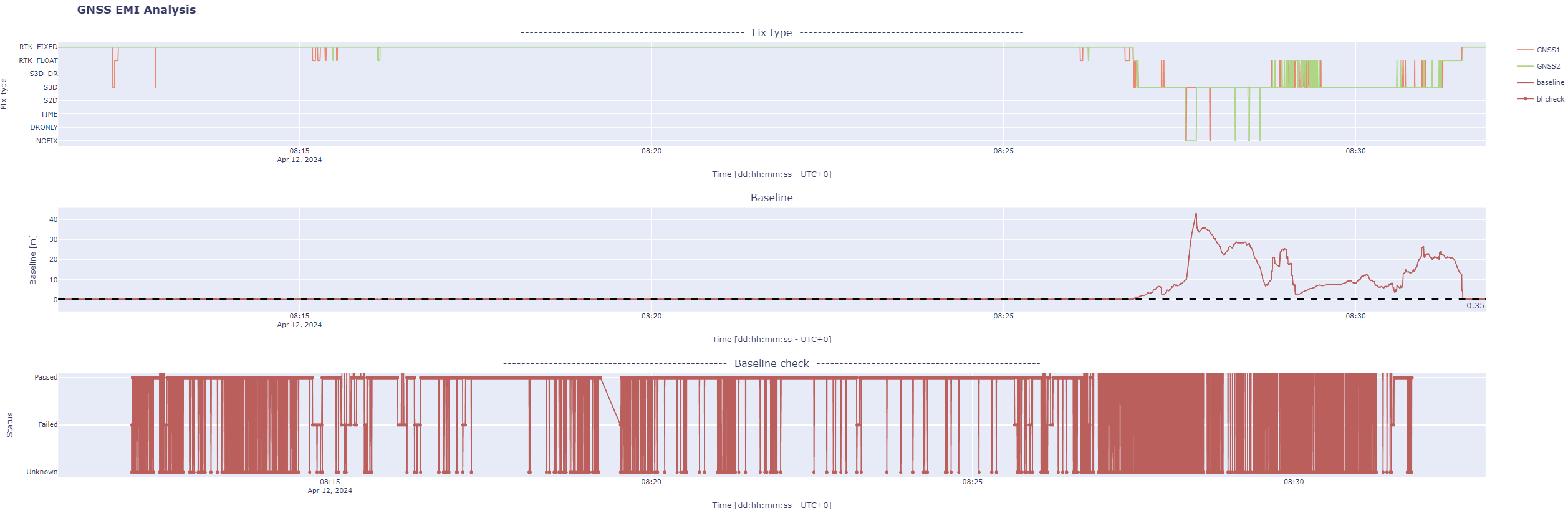
Fig. 1: GNSS fix type, estimated baseline, and baseline check plots.
The fourth plot presents a spectrum analysis graph for each L-band generated from the UBX-MON-SPAN messages of each GNSS receiver. The user can use this plot to detect patterns of electromagnetic interference affecting the GNSS signals. The left column presents the L1 and L2 bands for the GNSS1 receiver, while the right column presents this information for the GNSS2 receiver. The plots are centered at the frequencies of each L-band, where the L1 band operates at 1575.42 MHz and the L2 band at 1227.60 MHz. The user can use the slider at the bottom of the plot to move through time slides. Note that the maximum duration of this plot is 500 seconds. This plot will not contain information after this initial period.
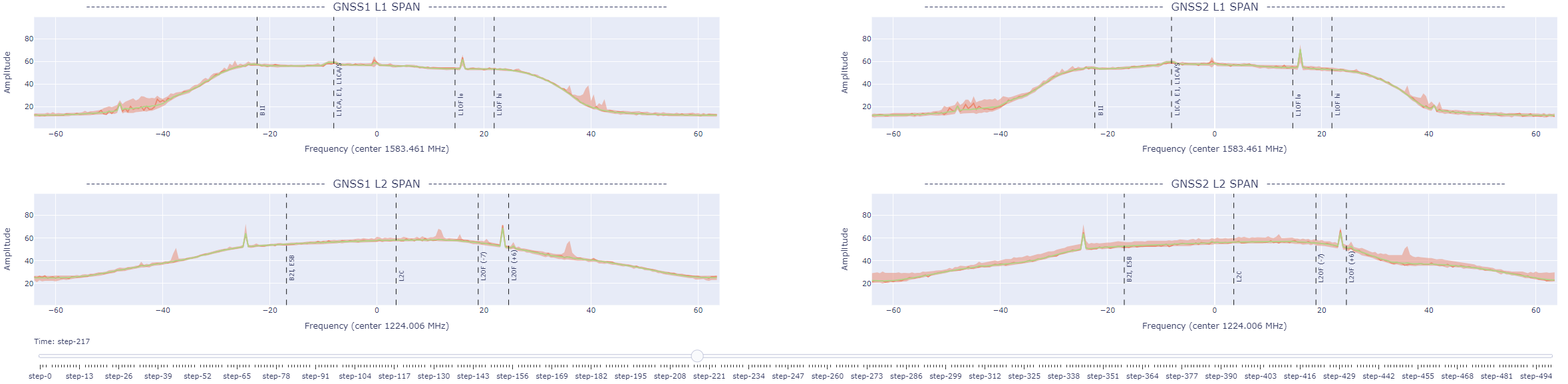
Fig. 2: Spectrum analysis graph for the L-bands of each GNSS receiver.
Expected results
Ideally, the estimated baseline should be accurate when both receivers are under RTK fixed conditions. However, it is known that the GNSS receivers can sometimes experience a 'false RTK fixed'. Thus, the user cannot entirely rely on the GNSS fix quality to assess performance. For the user to evaluate the sensor's performance, it is crucial to correlate the GNSS fix quality with the baseline check.
When operating under RTK fixed conditions, the baseline check should always pass. Ensuring the input GNSS extrinsics are accurate is crucial, as any discrepancy can lead to a failed baseline check. In addition, ensure the GNSS antennas are not obstructed by obstacles or affected by electromagnetic noise and that the selected basestation is nearby (less than 25 km away).
If the baseline check fails, the Vision-RTK 2's position output will not experience a jump.
Examples
In GNSS-degraded scenarios, the reported baseline might be wrong by several meters, which can affect the scale of the plot, as shown in Fig. 6. You can always zoom in on the Y-axis only to aid in visualizing the performance of the baseline estimate when the sensor is under RTK fixed conditions.
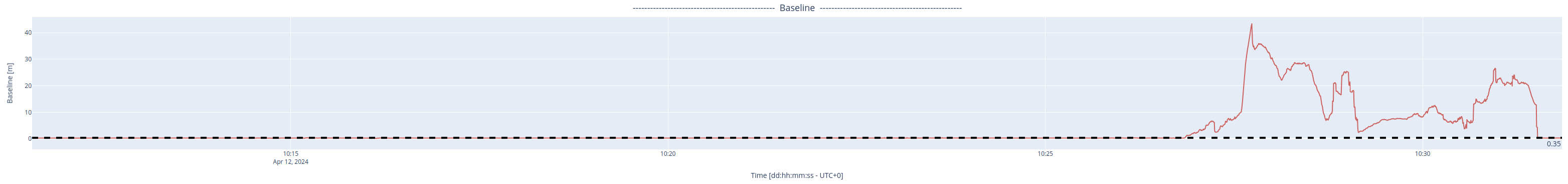
Fig. 8: Estimated baseline plot without zooming in on the Y-axis.
When entering a GNSS outage, the estimated baseline might present a "spike", where the baseline is hundreds of meters, as shown in Fig. 12. This is the expected behavior of the GNSS receivers.
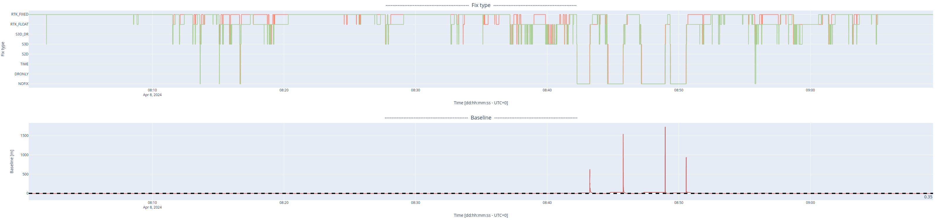
Fig. 12: Spikes in the estimated baseline of the GNSS receivers when entering a GNSS outage.
Under ideal conditions, the spectrum graph will show a smooth rectangular shape on both L-bands. Some noise is to be expected when the platform is moving, as shown in Fig. 13, due to GNSS signals being reflected from nearby buildings or other objects and some devices in the environment generating weak electromagnetic fields that slightly affect the GNSS signals in the area without entirely disrupting them.
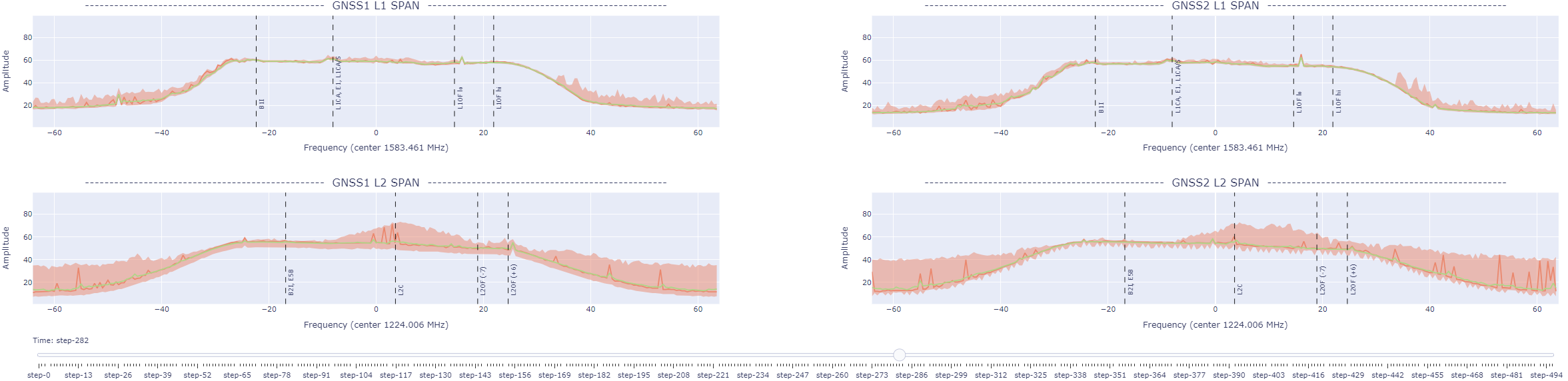
Fig. 13: Environmental electromagnetic noise observed in the spectrum graph.
However, the presence of a powerful source of electromagnetic fields in close proximity to the GNSS antennas can lead to a complete disruption of the GNSS signals in the area. This disruption is clearly visible in the spectrum graph, as shown in Fig. 14. The figure illustrates the spectrum graph of a sensor affected by a LiDAR placed near the GNSS antennas. The electromagnetic field produced by its motor can significantly disrupt the L2 band of the GNSS receiver, thereby affecting the time required to obtain an RTK-fixed measurement and the quality of the position estimate.
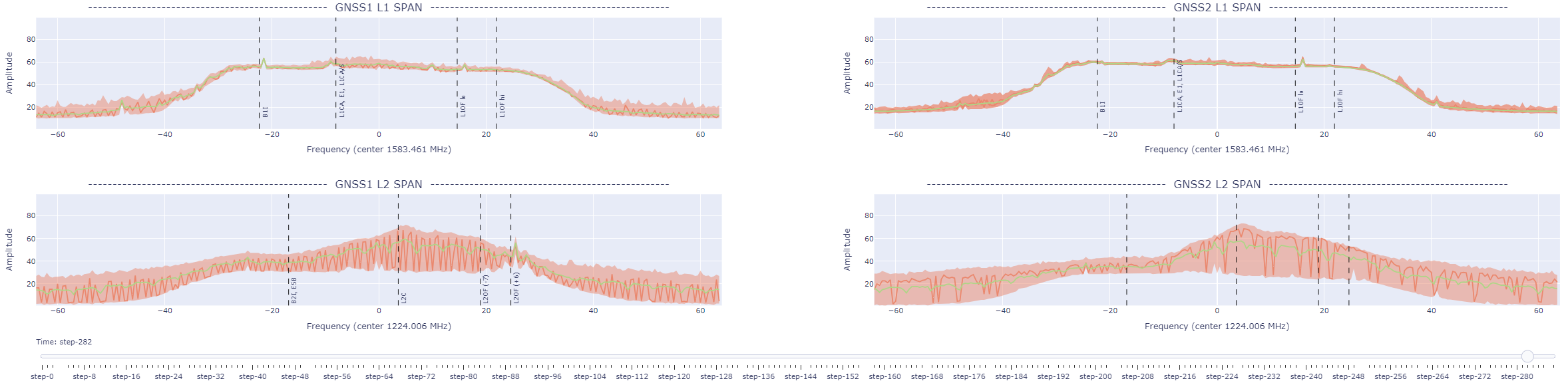
Fig. 14: Interference pattern caused by a nearby LiDAR in the spectrum graph.
Similarly, Fig. 15 presents the noise generated by a nearby USB-3 device. Unshielded cables and USB-3 ports can generate strong electromagnetic fields that disrupt nearby GNSS signals.
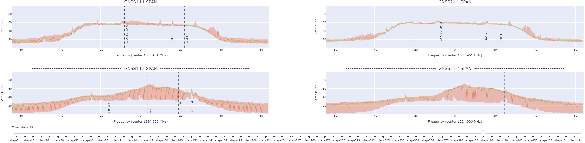
Fig. 15: Interference pattern caused by a nearby USB-3 port in the spectrum graph.
Further analysis
If the GNSS receivers experience issues obtaining an RTK fixed status or the estimated baseline is wrong under RTK fixed conditions, verify that the selected basestation is less than 15 km from the rover. The sensor might experience degraded performance if the selected RTK basestation is slightly far away (> 15 km). The sensor will experience degraded performance and difficulties computing an RTK-fixed solution if the basestation is excessively far away (> 25 km). In this case, please choose a different NTRIP mountpoint or re-connect to the VRS service.
If the signal-to-noise ratio is low throughout the recording (i.e., CN0 under 42 dBHz), check the integrity of the GNSS cables and the power supply to the GNSS antennas, and ensure no objects are obstructing the GNSS antennas' view or any electromagnetic interference is affecting them.
Use shielded cables only and avoid sources of electromagnetic interference near the antennas (e.g., LiDAR, USB3).